Ural River Flood Mapping: Data Acquisition in GEE and Visualization in QGISКартирование паводков реки Урал: получение данных в GEE и визуализация в QGIS
This project maps the maximum spring flood extent along the Ural River in West Kazakhstan for April 2024 and April 2025. The workflow consists of two steps: acquiring and processing satellite data in Google Earth Engine, then importing and styling the results in QGIS for cartographic output.
Background
Spring flooding along the Ural River is a recurring phenomenon in West Kazakhstan. Each year, snowmelt in upstream areas causes significant water level rise, affecting settlements, agricultural land, and infrastructure across the region.
Part 1 — Data acquisition in Google Earth Engine
Why MNDWI instead of NDWI
The classic NDWI uses Green and NIR bands, but MNDWI replaces NIR with SWIR (B11), which suppresses built-up land noise better and improves water detection in vegetated and urban areas:
MNDWI = (Green − SWIR) / (Green + SWIR)
Values above 0.2 indicate open water. The script applies this threshold to each image and takes the .max() composite to capture the widest flood extent over the selected period.
Cloud masking
Instead of a simple CLOUDY_PIXEL_PERCENTAGE filter, the script joins the Sentinel-2 collection with COPERNICUS/S2_CLOUD_PROBABILITY and masks pixels where cloud probability exceeds 50%. This gives per-pixel cloud removal rather than image-level filtering, resulting in much cleaner composites.
⚠ Large area warning: GEE may throw a "Computation timed out" or "Export too large" error if your geometry covers a very large region. If this happens — increase scale (e.g. from 10 to 30) or split the area into smaller tiles.
var area = geometry; // draw your field of study in GEE
var startDate = '2024-04-15';
var endDate   = '2024-05-15';

function addMNDWI(image) {
  var mndwi = image.normalizedDifference(['B3', 'B11']).rename('MNDWI');
  var waterMask = mndwi.gt(0.2).rename('water');
  return image.addBands(mndwi).addBands(waterMask)
    .copyProperties(image, ['system:time_start', 'system:index']);
}

var s2 = ee.ImageCollection('COPERNICUS/S2_SR_HARMONIZED')
  .filterBounds(area)
  .filterDate(startDate, endDate)
  .filter(ee.Filter.lt('CLOUDY_PIXEL_PERCENTAGE', 30));

var s2Cloud = ee.ImageCollection('COPERNICUS/S2_CLOUD_PROBABILITY')
  .filterBounds(area)
  .filterDate(startDate, endDate);

var joined = ee.ImageCollection(
  ee.Join.saveFirst('cloud_prob').apply(
    s2, s2Cloud,
    ee.Filter.equals({
      leftField: 'system:index',
      rightField: 'system:index'
    })
  )
);

var s2Collection = joined.map(function(image) {
  var mask = ee.Image(image.get('cloud_prob'))
    .select('probability').lt(50);
  return image.updateMask(mask)
    .divide(10000)
    .clip(area)
    .copyProperties(image, ['system:time_start', 'system:index']);
}).map(addMNDWI);

print('Total images:', s2Collection.size());

s2Collection
  .map(function(img) {
    return img.set('date_str',
      ee.Date(img.get('system:time_start')).format('YYYY-MM-dd'));
  })
  .aggregate_array('date_str')
  .distinct()
  .evaluate(function(dates, error) {
    if (error) { print('Date error: ' + error); return; }
    if (!dates || dates.length === 0) {
      print('No dates found — collection is empty');
      return;
    }
    print('Available dates (' + dates.length + '):');
    dates.sort().forEach(function(d) { print('  ' + d); });
  });

var maxFlood = s2Collection.select('water').max().unmask(0).clip(area);

var maxFloodArea = maxFlood.multiply(ee.Image.pixelArea()).rename('area');

var stats = maxFloodArea.reduceRegion({
  reducer: ee.Reducer.sum(),
  geometry: area,
  scale: 20,
  maxPixels: 1e13,
  bestEffort: true
}).getInfo();

var m2 = (stats && stats.hasOwnProperty('area')) ? stats['area'] : 0;
print('Flood zone total');
print('Area: ' + (m2 / 1e6).toFixed(2) + ' km²');
print('Area: ' + (m2 / 1e4).toFixed(1) + ' ha');

Map.centerObject(area, 10);
Map.addLayer(area, {color: 'FFFF00'}, 'AOI', true, 0.2);
Map.addLayer(maxFlood.selfMask(), {palette: ['0077b6']}, 'Flooded areas');

Export.image.toDrive({
  image: maxFlood.clip(area),
  description: 'flood_april_2024',  // rename as needed
  scale: 10,
  region: area,
  maxPixels: 1e13,
  folder: 'GEE_exports',
  fileFormat: 'GeoTIFF',
  crs: 'EPSG:32640' // UTM Zone 40N for Western Kazakhstan
});
Draw a polygon over your study area — it will be named geometry by default
Paste the script and click Run
Check the Console for image count, dates, and area statistics
Click Tasks tab → Run export to save the GeoTIFF to Google Drive
Tips & common issues
💡 Empty collection: If print('Total images:') returns 0, try expanding the date range or increasing CLOUDY_PIXEL_PERCENTAGE to 50–80.
⚠ "Export too large" error: GEE limits exports to 1e8 pixels by default. For large AOIs at 10 m resolution this is easily exceeded. Solutions:
Increase scale from 10 to 20 or 30
maxPixels: 1e13 is already set — that's the GEE maximum
If it still fails — split your AOI into smaller tiles manually
Use bestEffort: true in reduceRegion — it auto-adjusts scale
⚠ "Computation timed out": GEE has a limit on interactive computations. If getInfo() hangs — move the stats calculation inside an evaluate() callback, or run it as an Export task instead.
💡 CRS note:EPSG:32640 is UTM Zone 40N, appropriate for Western Kazakhstan. Change to your local UTM zone if working in a different region.
Part 2 — Visualization in QGIS
Importing the GeoTIFF
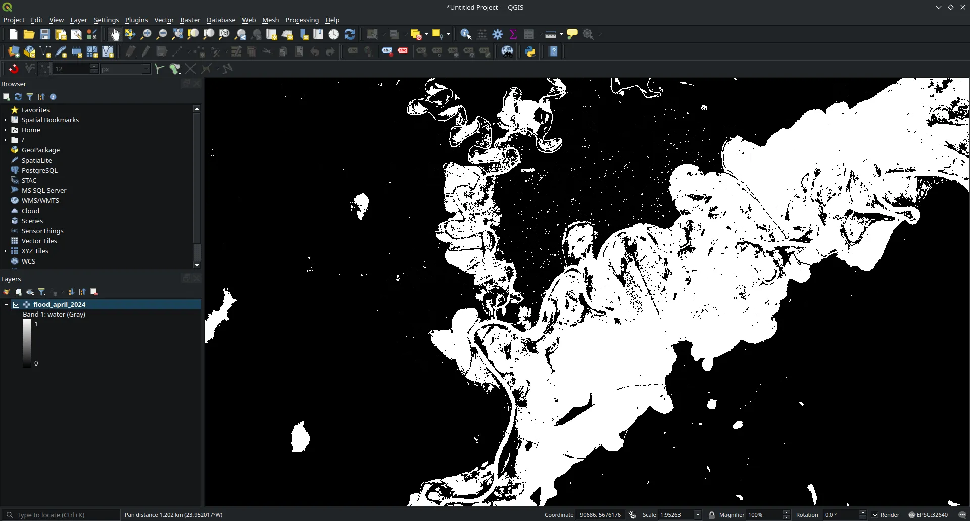
Once you have the exported .tif file from Google Drive, drag it into QGIS or use Layer → Add Layer → Add Raster Layer. By default the layer will appear in grayscale with values 0 (no water) and 1 (water) — it needs to be styled to become readable.
Styling the water layer
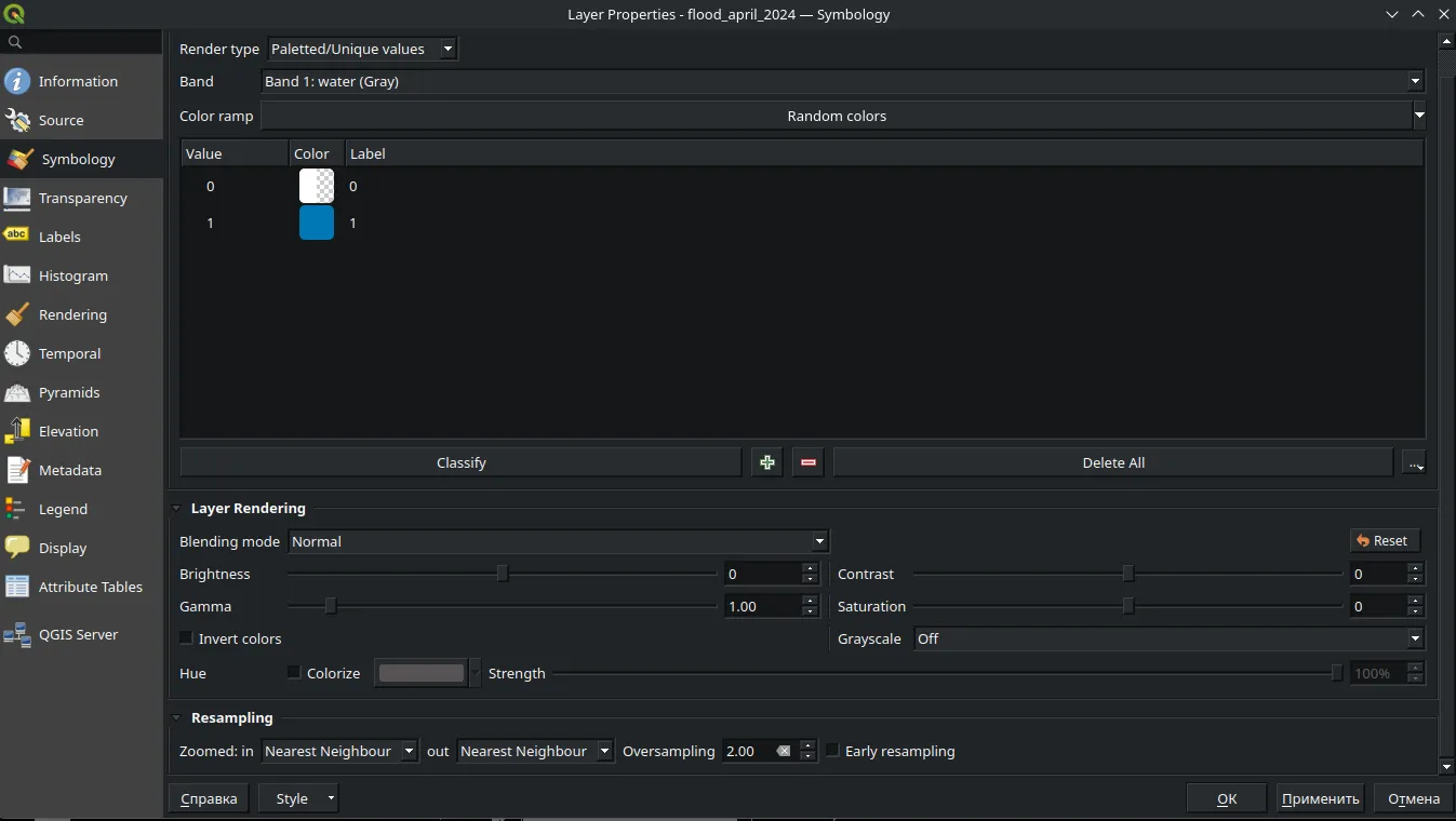
Right-click on your raster layer Layer Properties → Symbology. Since the raster is binary (0/1), switch the render type to Paletted/Unique values and classify. Assign value 1 (water) a solid blue color (e.g. #0077b6) and set value 0 to fully transparent so the basemap shows through.
Symbology settings: value 1 = blue, value 0 = transparent
Making it presentable
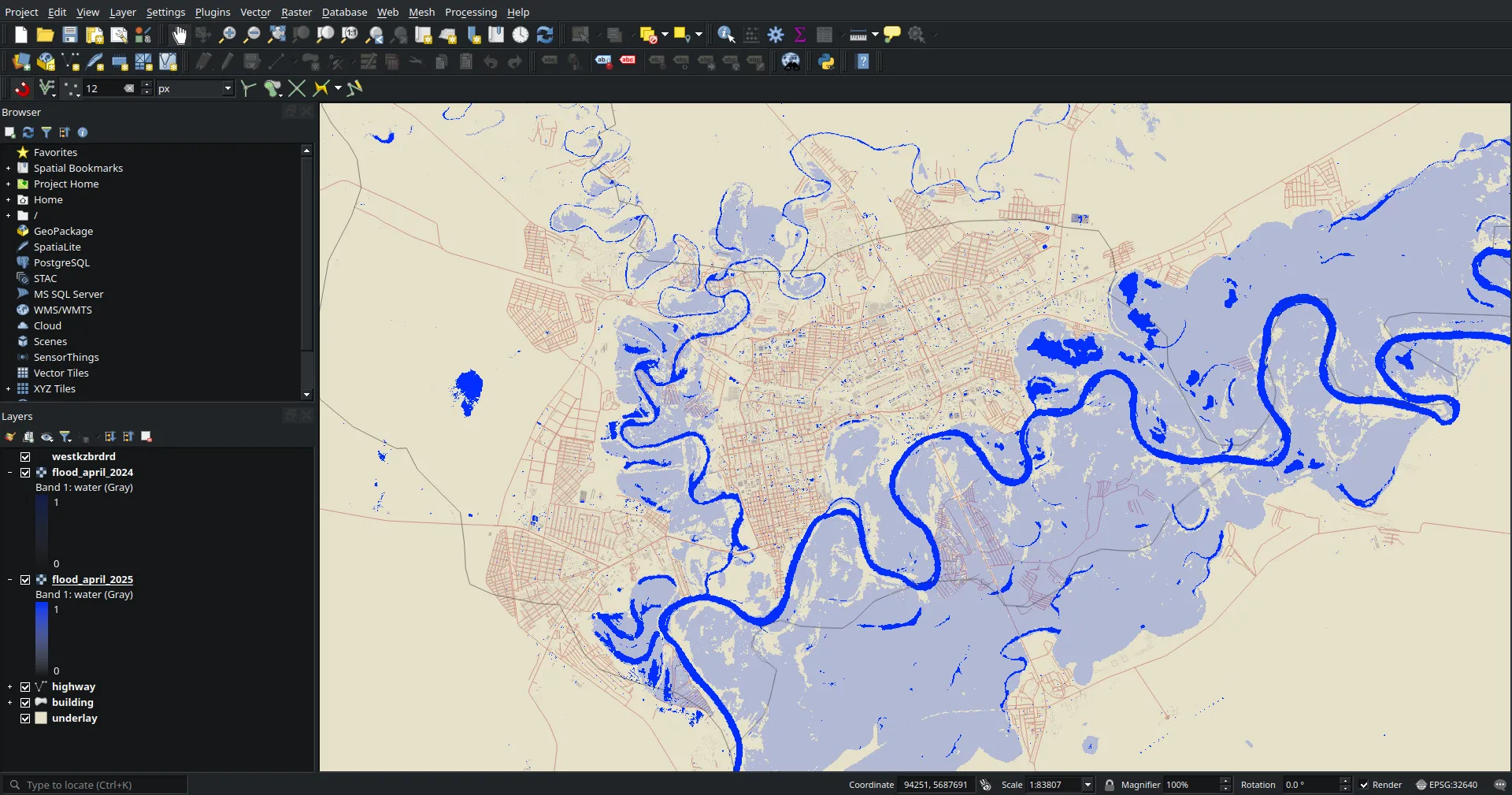
Add a basemap (e.g. OpenStreetMap via QuickMapServices plugin) beneath the flood layer for context. In the Print Layout, add a scale bar, north arrow, legend, and title. Export as PNG or PDF for the final map.
Styled flood extent over OpenStreetMap basemap
Results
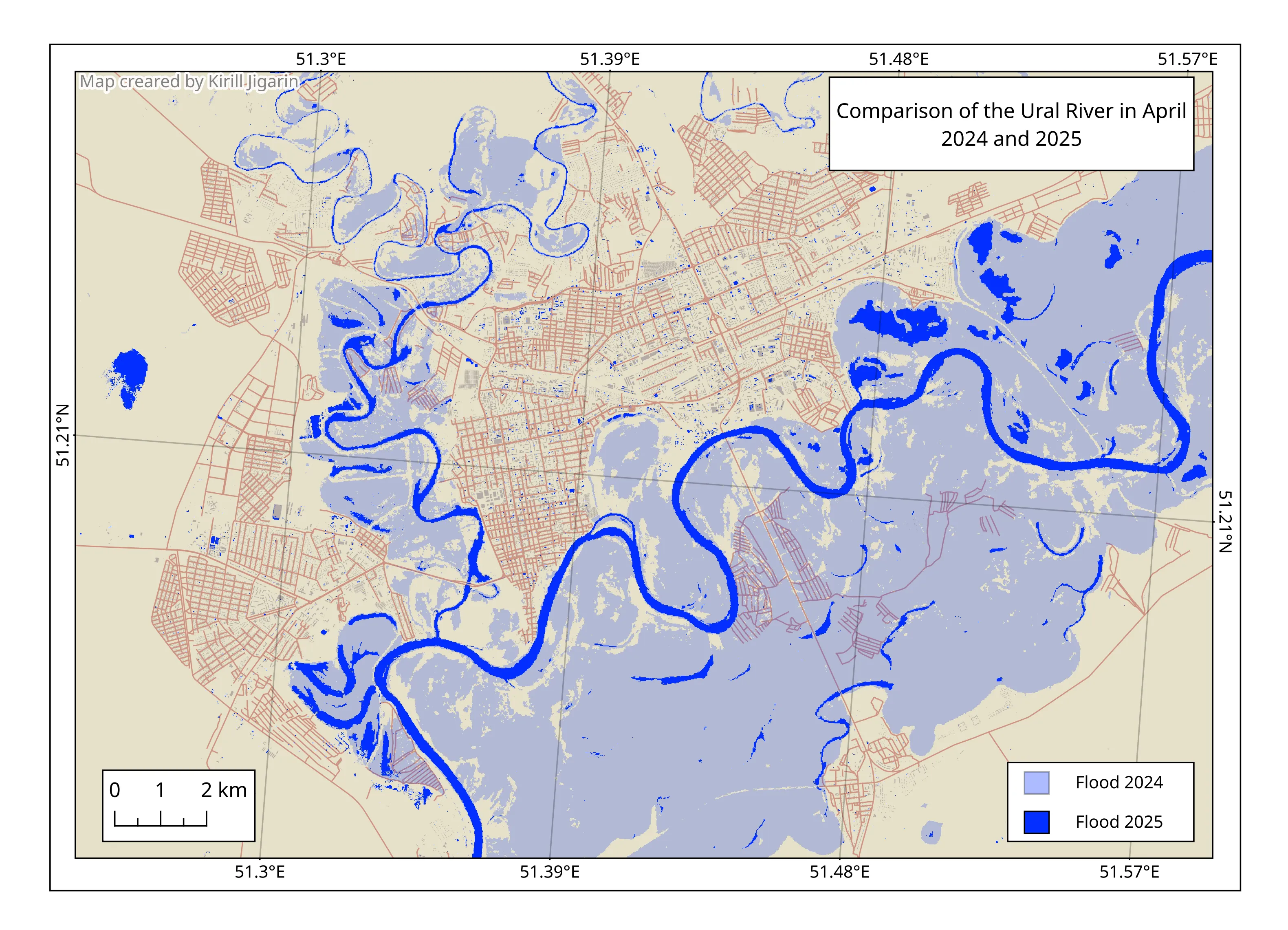
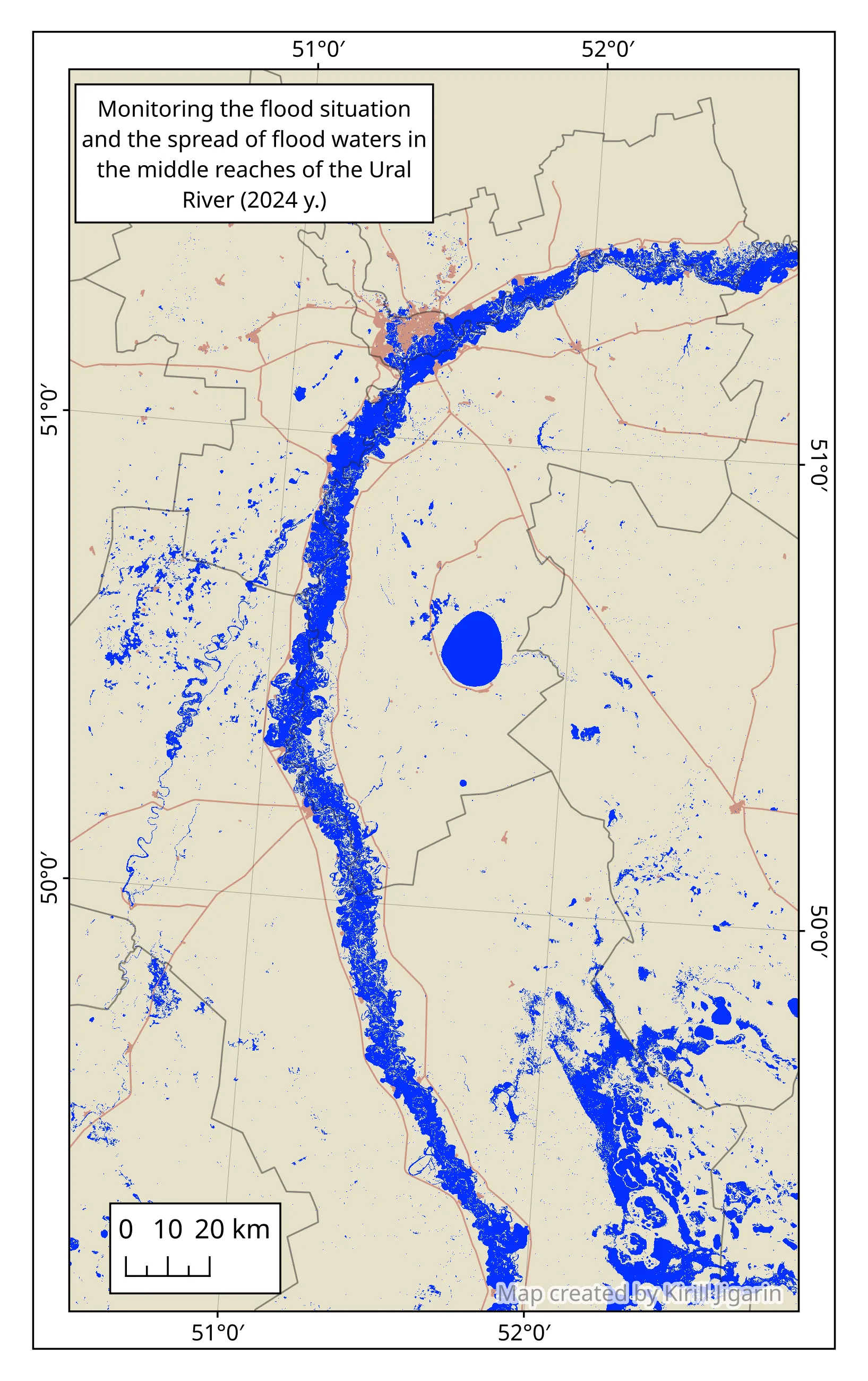
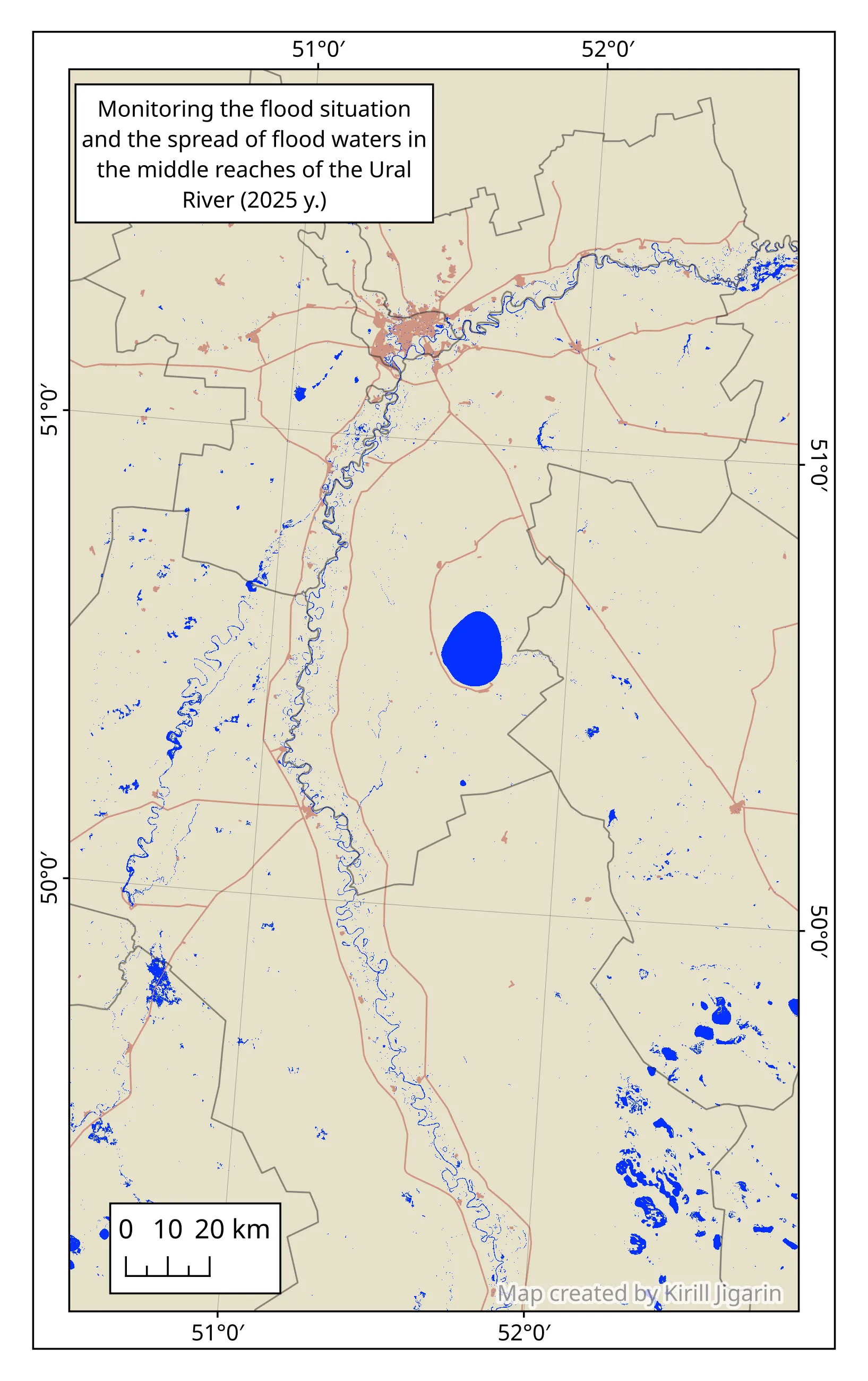
The maps below show the maximum flood extent for April 2024 and April 2025. The flood zone boundaries were derived from the MNDWI water mask exported from GEE and styled in QGIS.
Conclusion
Remote sensing tools allow rapid and accurate monitoring of flood dynamics. The combination of Google Earth Engine for data acquisition and QGIS for cartographic styling provides an efficient, reproducible workflow for mapping flood extents from freely available Sentinel-2 imagery.
Этот проект посвящён картированию максимальных масштабов весеннего паводка на реке Урал в Западном Казахстане за апрель 2024 и апрель 2025 года. Рабочий процесс состоит из двух этапов: получение и обработка спутниковых данных в Google Earth Engine, затем импорт и оформление результатов в QGIS для создания картографического продукта.
Контекст
Весеннее половодье на реке Урал — повторяющееся явление для Западного Казахстана. Ежегодно таяние снега в верховьях реки вызывает значительный подъём уровня воды, что затрагивает населённые пункты, сельскохозяйственные угодья и инфраструктуру региона.
Часть 1 — Получение данных в Google Earth Engine
Почему MNDWI, а не NDWI
Классический NDWI использует зелёный и ближний инфракрасный каналы, но в MNDWI ближний ИК заменён на SWIR (B11), что лучше подавляет шум от застроенных территорий и повышает точность обнаружения воды в вегетированных и городских зонах:
MNDWI = (Green − SWIR) / (Green + SWIR)
Значения выше 0.2 соответствуют открытой воде. Скрипт применяет этот порог к каждому снимку и берёт композит .max(), чтобы зафиксировать максимальную площадь затопления за выбранный период.
Маскировка облаков
Вместо простого фильтра CLOUDY_PIXEL_PERCENTAGE скрипт объединяет коллекцию Sentinel-2 с COPERNICUS/S2_CLOUD_PROBABILITY и маскирует пиксели, где вероятность облачности превышает 50%. Это обеспечивает попиксельное удаление облаков, а не фильтрацию на уровне целых снимков, что даёт значительно более чистые композиты.
⚠ Предупреждение о большой области: GEE может выдать ошибку «Computation timed out» или «Export too large», если полигон охватывает очень большую территорию. В этом случае увеличьте scale (например, с 10 до 30) или разбейте область на более мелкие тайлы.
var area = geometry; // нарисуйте полигон исследуемой области в GEE
var startDate = '2024-04-15';
var endDate   = '2024-05-15';

function addMNDWI(image) {
  var mndwi = image.normalizedDifference(['B3', 'B11']).rename('MNDWI');
  var waterMask = mndwi.gt(0.2).rename('water');
  return image.addBands(mndwi).addBands(waterMask)
    .copyProperties(image, ['system:time_start', 'system:index']);
}

var s2 = ee.ImageCollection('COPERNICUS/S2_SR_HARMONIZED')
  .filterBounds(area)
  .filterDate(startDate, endDate)
  .filter(ee.Filter.lt('CLOUDY_PIXEL_PERCENTAGE', 30));

var s2Cloud = ee.ImageCollection('COPERNICUS/S2_CLOUD_PROBABILITY')
  .filterBounds(area)
  .filterDate(startDate, endDate);

var joined = ee.ImageCollection(
  ee.Join.saveFirst('cloud_prob').apply(
    s2, s2Cloud,
    ee.Filter.equals({
      leftField: 'system:index',
      rightField: 'system:index'
    })
  )
);

var s2Collection = joined.map(function(image) {
  var mask = ee.Image(image.get('cloud_prob'))
    .select('probability').lt(50);
  return image.updateMask(mask)
    .divide(10000)
    .clip(area)
    .copyProperties(image, ['system:time_start', 'system:index']);
}).map(addMNDWI);

print('Total images:', s2Collection.size());

s2Collection
  .map(function(img) {
    return img.set('date_str',
      ee.Date(img.get('system:time_start')).format('YYYY-MM-dd'));
  })
  .aggregate_array('date_str')
  .distinct()
  .evaluate(function(dates, error) {
    if (error) { print('Date error: ' + error); return; }
    if (!dates || dates.length === 0) {
      print('No dates found — collection is empty');
      return;
    }
    print('Available dates (' + dates.length + '):');
    dates.sort().forEach(function(d) { print('  ' + d); });
  });

var maxFlood = s2Collection.select('water').max().unmask(0).clip(area);

var maxFloodArea = maxFlood.multiply(ee.Image.pixelArea()).rename('area');

var stats = maxFloodArea.reduceRegion({
  reducer: ee.Reducer.sum(),
  geometry: area,
  scale: 20,
  maxPixels: 1e13,
  bestEffort: true
}).getInfo();

var m2 = (stats && stats.hasOwnProperty('area')) ? stats['area'] : 0;
print('Flood zone total');
print('Area: ' + (m2 / 1e6).toFixed(2) + ' km²');
print('Area: ' + (m2 / 1e4).toFixed(1) + ' ha');

Map.centerObject(area, 10);
Map.addLayer(area, {color: 'FFFF00'}, 'AOI', true, 0.2);
Map.addLayer(maxFlood.selfMask(), {palette: ['0077b6']}, 'Flooded areas');

Export.image.toDrive({
  image: maxFlood.clip(area),
  description: 'flood_april_2024',
  scale: 10,
  region: area,
  maxPixels: 1e13,
  folder: 'GEE_exports',
  fileFormat: 'GeoTIFF',
  crs: 'EPSG:32640'
});
Нарисуйте полигон исследуемой области — по умолчанию он будет называться geometry
Вставьте скрипт и нажмите Run
Проверьте в консоли количество снимков, доступные даты и площадь затопления
Перейдите на вкладку Tasks → запустите экспорт для сохранения GeoTIFF на Google Drive
Советы и типичные ошибки
💡 Пустая коллекция: Если print('Total images:') возвращает 0 — расширьте диапазон дат или увеличьте CLOUDY_PIXEL_PERCENTAGE до 50–80.
⚠ Ошибка "Export too large": GEE ограничивает экспорт до 1e8 пикселей. Для больших областей на разрешении 10 м этот лимит легко превышается. Решения:
Увеличьте scale с 10 до 20 или 30
maxPixels: 1e13 уже задан — это максимум для GEE
Если ошибка сохраняется — вручную разбейте область на тайлы
Используйте bestEffort: true в reduceRegion — он автоматически подбирает масштаб
⚠ "Computation timed out": GEE ограничивает интерактивные вычисления по времени. Если getInfo() зависает — перенесите расчёт статистики внутрь колбэка evaluate() или запустите как задачу Export.
💡 Система координат:EPSG:32640 — это UTM Zone 40N, подходящий для Западного Казахстана. При работе в другом регионе выберите соответствующую зону UTM.
Часть 2 — Визуализация в QGIS
Импорт GeoTIFF
После того как файл .tif скачан с Google Drive, перетащите его в QGIS или используйте Слой → Добавить слой → Добавить растровый слой. По умолчанию слой отобразится в оттенках серого со значениями 0 (нет воды) и 1 (вода) — его нужно настроить, чтобы карта стала читаемой.
Сырой GeoTIFF после импорта черно-белый, когда стиль ещё не настроен
Настройка стиля водного слоя
Нажмите правой кнопкой мыши по вашему растровому слою Свойства слоя → Стиль. Поскольку растр бинарный (0/1), переключите тип рендера на Уникальные значения и выполните классификацию. Назначьте значению 1 (вода) сплошной синий цвет (например, #0077b6), а значение 0 сделайте полностью прозрачным — так будет видна подложка.
Настройки стиля: значение 1 = синий, значение 0 = прозрачный
Финальное оформление
Добавьте подложку (например, OpenStreetMap через плагин QuickMapServices) под слой затопления для контекста. В макете печати добавьте масштабную линейку, стрелку севера, легенду и заголовок. Экспортируйте в PNG или PDF для получения готовой карты.
Зона затопления со стилем
Результаты
Карты ниже показывают максимальную площадь затопления за апрель 2024 и апрель 2025 года. Границы зон затопления получены из маски воды MNDWI, экспортированной из GEE и оформленной в QGIS.
Заключение
Средства дистанционного зондирования позволяют быстро и точно отслеживать динамику наводнений. Связка Google Earth Engine для получения данных и QGIS для картографического оформления обеспечивает эффективный и воспроизводимый рабочий процесс картирования паводков на основе бесплатных снимков Sentinel-2.